training locomotion policies for a quadruped

Legged locomotion is one of the most researched problems in the physical AI space. Balancing legged robots is hard enough and making the controllers generalizable to difficult terrains is even harder. This is why I set out to train a reinforcement policy that enabled a quadruped to walk in challenging terrains.

I was really inspired by a paper I read earlier in the year:

Dynamics and Domain Randomized Gait Modulation with Bezier Curves for Sim-to-Real Legged Locomotion by Rahme et al.

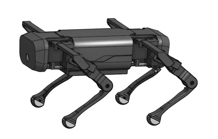
Building off of this I decided to use the URDF from an open-source robot, Open Quadruped, designed by Adham Elewaraby.

Overview of the Controller

End-to-End ML systems have been gaining a lot of traction in the field but I decided to go down the route of mixing traditional control and learned policies in order to develop the gait. I developed a baseline controller using a trajectory generator into an inverse kinematics module. I then wrapped this in a policy that adjusts the parameters of the trajectory generator to handle more varied terrain in real-time.

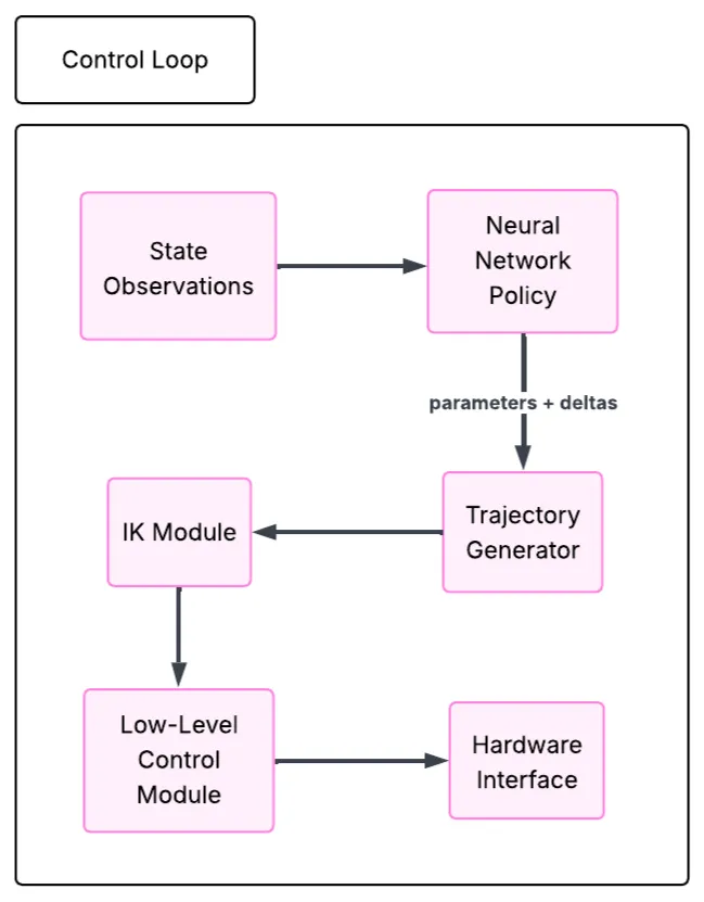
Baseline Controller

This controller is split into 2 parts: the trajectory generator and the inverse kinematics

Bezier Curve Based Trajectory Generator: The gait is just the timing and motion profile of the legs that generate some desired movement. There are 2 phases to the gait: the swing phase and the support phase. The swing phase is the forward movement that occurs in the air. The support phase is the backward movement into the ground that brings the leg back to its neutral stance.

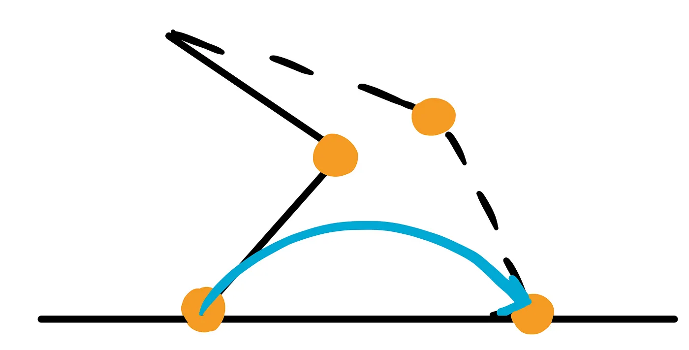
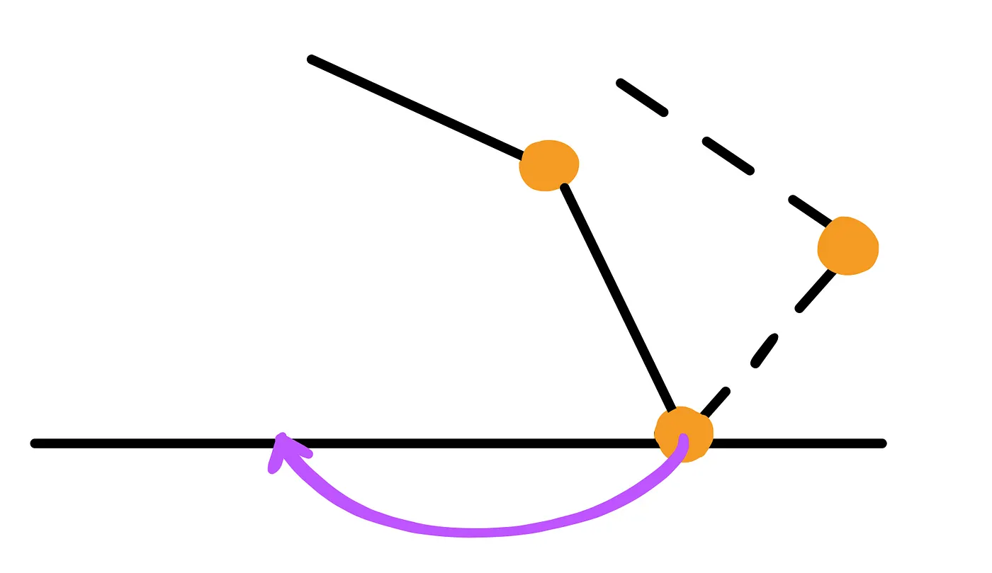
As seen above, after this cycle of swing phase into the support phase the leg moves forward and returns to its initial configuration. I represented the curves using bezier curves. The gist of bezier curves is essentially the process of stacking linear interpolations on top of each other to form more complex curves. A linear interpolation is the following equation:

$$P(t) = (1 - t)P_0 + tP_1, \quad t \in [0,1]$$

To extend this into a quadratic bezier curve we can nest 2 of these interpolations between 3 points to get a curve between 2 points:

$$\begin{aligned}a(t) &= (1 - t)P_0 + tP_1 \\b(t) &= (1 - t)P_1 + tP_2 \\P(t) &= (1 - t)a(t) + tb(t)\end{aligned}$$

This maps out a curve that looks like this:

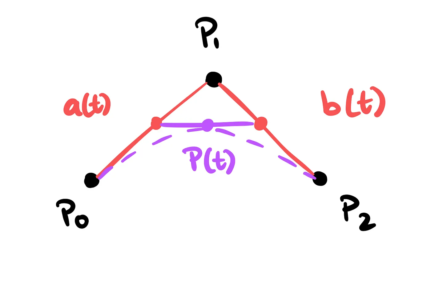
That equation for P(t) can be simplified to:

$$P(t) = P_0 + t(-2P_0 + 2P_1) + t^2(P_0 - 2P_1 + P_2)$$

In matrix form:

$$P(t) =\begin{bmatrix}1 & t & t^2\end{bmatrix}\begin{bmatrix}1 & 0 & 0 \\-2 & 2 & 0 \\1 & -2 & 1\end{bmatrix}\begin{bmatrix}P_0 \\P_1 \\P_2\end{bmatrix}$$

These curves are parameterized based on three physical parameters:

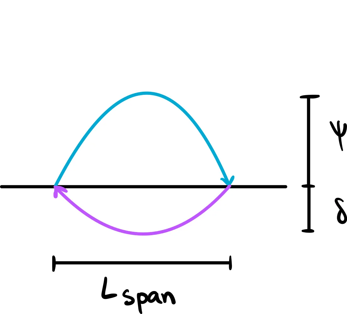
where $\psi$ is the clearance height, $\delta$ is the ground penetration, and $L_{span}$ is the length of the stride

The matrix form can then be used to represent the swing phase with these 3 (x, z) points:

$$P_0 = (0,0) \quad P_1 = \left(\frac{L_{span}}{2}, \psi\right) \quad P_2 = (L_{span}, 0)$$

and the support phase with these 3 (x, z) points:

$$P_0 = (L_{span}, 0) \quad P_1 = \left(\frac{L_{span}}{2}, -\delta\right) \quad P_2 = (0,0)$$

We need to reparameterize the entire trajectory between [0. 1] where the swing phase is [0, 0.5] and the support phase is [0.5, 1]:

$$\begin{aligned}u_{swing} &= 2leg_{phase}, \ \mathrm{for}\ leg_{phase} \in [0,0.5) \\u_{support} &= 2(leg_{phase} - 0.5), \ \mathrm{for}\ leg_{phase} \in [0.5,1)\end{aligned}$$

where $u$ is the input into the respective curves.

Extending P(t) to include movement in the y-axis with a quick change:

Let the original point from the curve be $P_b(t) = (x_b, z_b)$. To move with a translation angle $\rho$:

$$P(t) = (x_b\cos(\rho), x_b\sin(\rho), z_b).$$

Yaw control is added by rotating each leg's neutral foot position by the desired yaw change over one gait period:

$$\theta = T_{gait}\omega$$

For a neutral foot position $(x,y)$, the resulting displacement is

$$\begin{aligned} d_x &= x\cos\theta - y\sin\theta - x \\ d_y &= x\sin\theta + y\cos\theta - y \end{aligned}$$

where the neutral positions are $(\pm L/2, \pm W/2)$, with signs determined by the leg. These displacements define a yaw Bézier trajectory with swing control points

$$Y_0=(0,0,0),\quad Y_1=\left(\frac{d_x}{2},\frac{d_y}{2},\psi\right),\quad Y_2=(d_x,d_y,0)$$

and support control points

$$Y_0=(d_x,d_y,0),\quad Y_1=\left(\frac{d_x}{2},\frac{d_y}{2},-\delta\right),\quad Y_2=(0,0,0)$$

The final foot trajectory is the sum of the translational and yaw components:

$$P_{final}(t)=P(t)+Y(t)$$

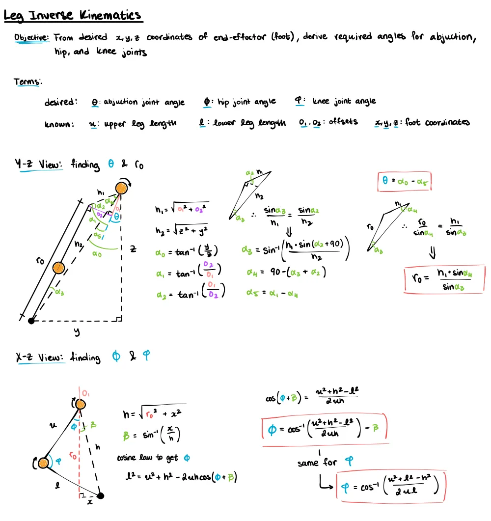
Inverse Kinematics Module: Because I control the quadruped via each leg individually, I derived the inverse kinematics for each leg individually with reference from its hip. Here is the full derivation:

Putting it Together With the trajectory generator and inverse kinematics defined, the final step is coordinating the four legs. For a trot gait, diagonal leg pairs are offset by half a gait cycle, so one pair is in swing while the other is in support. The phase of each leg is therefore:

$$leg_{phase} = (global_{phase} + phase_{offset}) \bmod 1$$

The trajectory generator and inverse kinematics are then combined in a loop to form the full controller. A PD correction is also used to maintain the desired heading and compensate for disturbances caused by mass imbalances and other unmodeled torques.

Designing the Environment

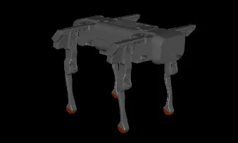
MuJoCo environments are based on XML and physical design of the world in simulation was quite simple since it’s just a platform that the robot would walk on. To bring the robot in all I had to do was convert the robot' URDF to a MJCF xml file using a standard converter. This was quite smooth except that the collision meshes on the feet had to be tweaked.

Domain and Dynamics Randomization: The most interesting thing I gained from the paper was their usage of dynamics and domain randomization within the environment. Domain, in this sense is referring to the actual environment the robot acts in, and Dynamics is referring to the physics governing the environment; things like friction, link masses, and gravity. There is a fundamental difference between the simulated world and the real world so training a policy in a singular simulated world would allow for those differences to really show up when deploying the policy in the real world. By randomizing the domain and dynamics you are essentially training the robot to be adaptable across thousands of potential worlds. This makes it so that bringing the robot into the real world is just 1 more of those worlds its already been able to adapt to.

The way I went about implementing this was in 2 ways:

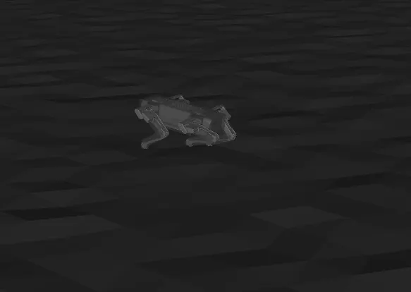
• Domain: I added a height map to the xml file which essentially took a set of x, y, z values that described the amplitudes of noise to add to the floor height and I randomly sampled values for this according to a gaussian distribution with a mean of 0.
• Dynamics: In a similar fashion to above I randomly sampled values to adjust the friction between the feet and the ground, as well as the masses of the various links within the robot. I centred the distribution around whatever values were in the original xml and then changed them before the rollout occurred

Observation Space: The robot is fitted with an IMU so the observation space was defined as a 10 dimensional space with the following quantities which were the same used by the paper:

1. Pitch
2. Roll
3. Yaw
4–6. Linear Accelerations: x, y, z
7–10. Phase of trajectory for each leg: FL, FR, BL, BR

Action Space: The policy essentially modulates the baseline controller loop so the action space is 14 dimensions for both positional offsets and parameter modulations into the trajectory generator:

1–12. dx, dy, dz for each leg end-effector
13. clearance height parameter
14. ground penetration parameter

Reward Function This was probably the part I spent the most time trying to get right because it starts off quite arbitrarily and requires tuning to get stable training. At first I tried using the reward structure from the original paper:

$$r_t = \Delta_x - 10(|r| + |p|) - 0.03\sum |\omega|$$

where $\Delta_{x}$ is the forward movement of the robot, $r$ is the roll angle, $p$ is the pitch angle, and $\omega$ is the vector of all angular velocities. Overall this reward formulation incentivized forward movement and then punished any other angular movement.

When I tried this however, it did not work very well and I am assuming this has to do with differences in the physics environment that I used compared to the paper. I had used MuJoCo and they had used PyBullet. With the original reward the robot learned to exploit the physics of the simulator and dig itself unrealistically into the ground and propel itself forward through the air. This is obviously undesired behaviour.

After a couple more iterations, some researching, and more testing I ended up using this reward function:

$$r_t = r_{forward} + 0.2r_{yaw} + 0.2r_{lateral} + 0.5r_{posture} + 0.1r_{shake} + r_{backward}$$

where

$$\begin{aligned}r_{forward} &= \exp\left(-\frac{(v_x - v_x^*)^2}{0.1}\right) \\r_{yaw} &= -|\omega_z - \omega_z^*| \\r_{lateral} &= -|v_y| \\r_{posture} &= -(|r| + |p|) \\r_{shake} &= -|a_z| \\r_{backward} &=\begin{cases}-2|v_x|, & \mathrm{if}\ v_x < 0 \\0, & \mathrm{otherwise}\end{cases}\end{aligned}$$

I modified the reward to incentivize the robot to follow a target forward velocity instead of plainly rewarding any forward movement. I did the same thing with the yaw rate. The lateral, posture, and shake terms serve to just penalize undesired movement. I added the backwards penalty because there were glitches in the physics of the environment causing the robot to jump backwards so I wanted to heavily penalize this behaviour during rollouts.

Model Architecture

Because this model would be ran on physical robots I wanted it to be as lightweight as possible while still being powerful which is why I chose a simple fully connected architecture:

$$10 \rightarrow 64 \rightarrow 14$$

Training

The training for this was quite straightforward because I utilized stable_baselines3 for the training algorithm since I was more interested in the building up the environment than implementing the algorithms from scratch. I used PPO because it is an extremely reliable algorithm. The policy was trained using a fixed gait, with parameters such as stride length, forward velocity, and yaw rate held constant throughout training. I followed this setup because the original paper found that policies trained under fixed gait conditions could still generalize to different gait parameters at deployment.

Results

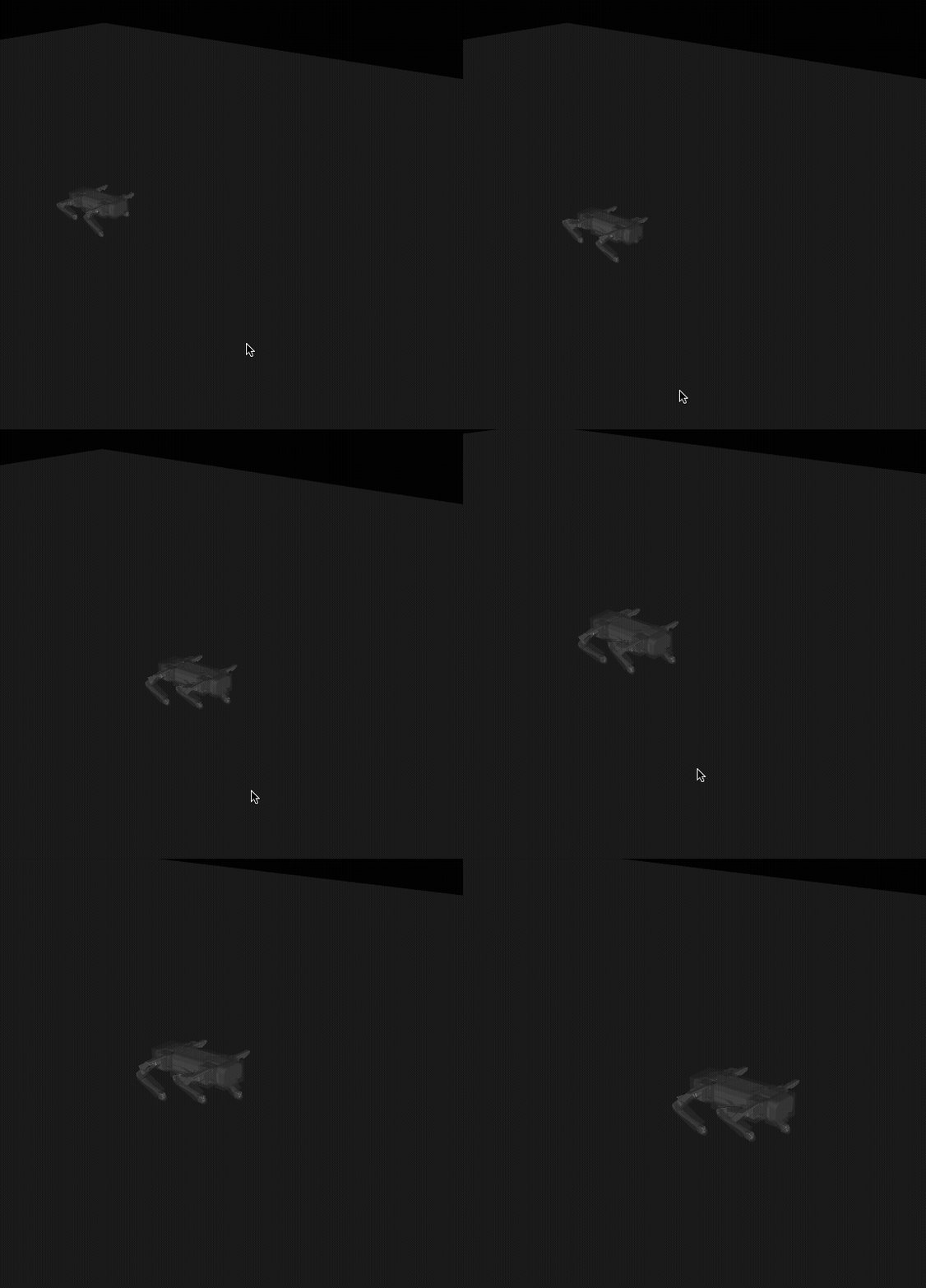
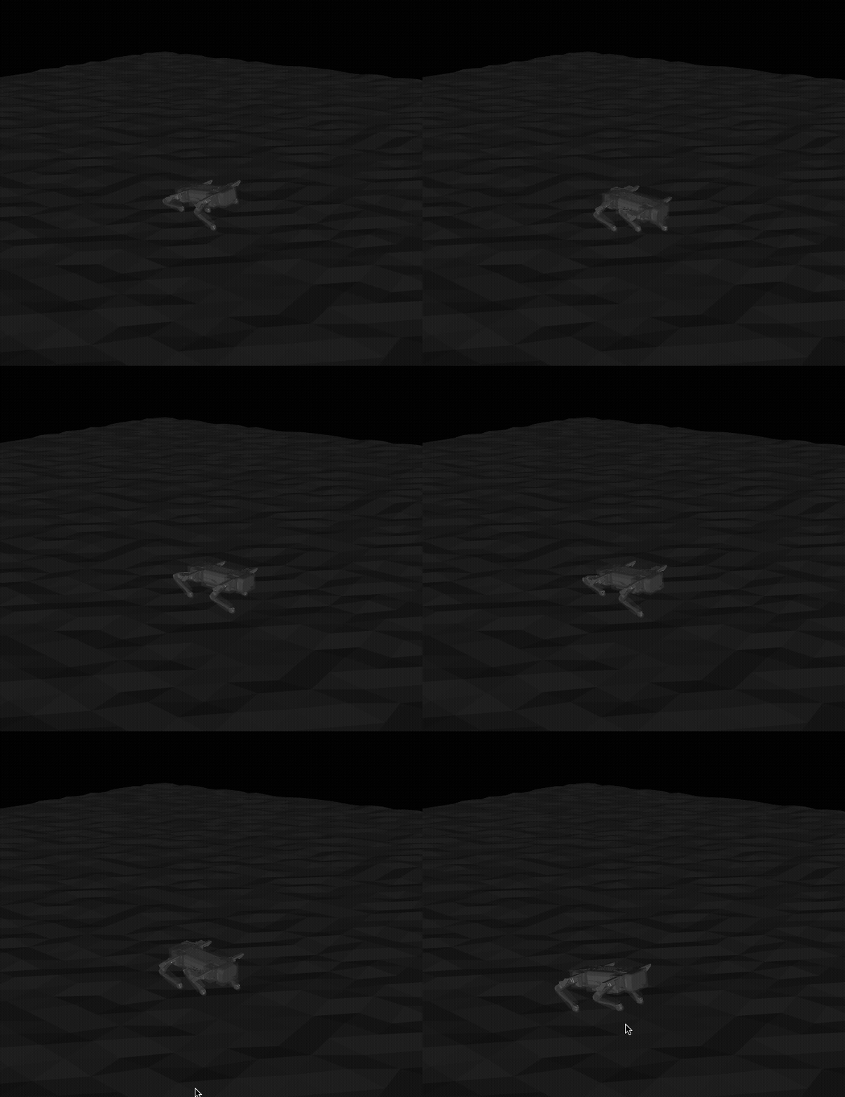
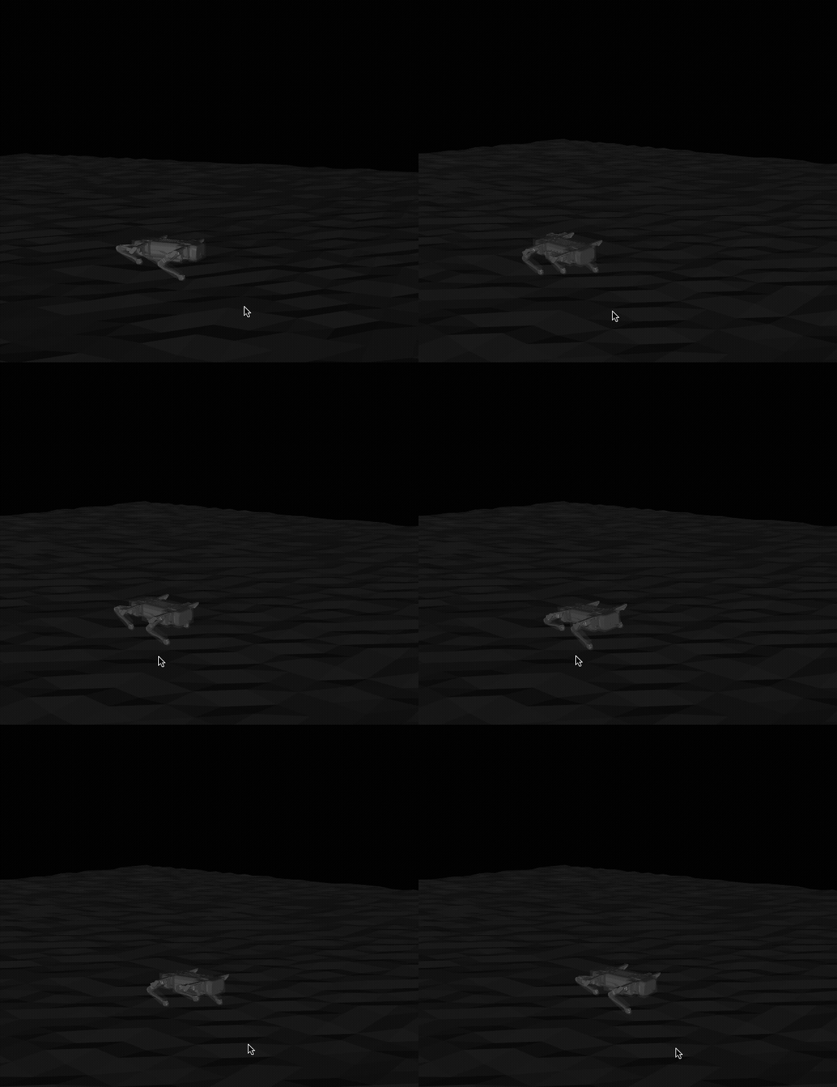
Before and after wrapping the controller with the policy:

Future Work

First and foremost I would love to deploy this policy on the physical quadruped which is something I am currently working on but the electrical for it is proving to be much harder than expected.

Beyond deploying on a physical robot however, there are a couple features I believe I could add in the future to improve the robustness of the policy or make the controller more effective:

• More gaits: gallops (4 legs in the air) , bounds (back together and front together), pace (side pairs together)
• More realistic terrain types: stairs, rocks, sand, ramps, etc.
• More complex trajectories other than simple quadratic curves like combining cubic curves to form complex splines