teaching a robot to understand the world with JEPA

Overview

Building on the JEPA-based latent world model introduced by Maes et al. (2026) in LeWorldModel, I extended the architecture to incorporate multi-view visual observations and robot proprioception. I then used the learned action-conditioned dynamics for latent-space planning, with a goal-conditioned actor seeding the MPC planner, forming a low-level controller for simulated lifting tasks.

Background / Motivation

World models have recently gained popularity as an alternative to behavioural cloning for learning robot manipulation policies. The premise of BC / Imitation Learning is that the policy learns mappings between observations at a given time step and the actions it should take. This has shown to be quite effective for specific tasks and, with enough scale, has even shown some ability to generalize. However, it does not explicitly model how the actions it takes impact the world.

World models offer an alternate approach. Rather than directly learning what actions to take given a state, they learn how actions impact the current state by training a neural network to predict the future state of the environment given the current state and an action. Once you can predict how actions change the environment, you can use methods such as model predictive control to search for actions that reach some goal state representing task completion.

JEPA (Joint-Embedding Predictive Architecture) models have emerged as one of the leading architectures to learn really effective world models. It was proposed by Yann LeCun who has been a strong proponent for world models when it comes to developing true physical intelligence. His essay/manifesto A Path Towards Autonomous Machine Intelligence is a really great read and dives really deep into why he believes world models are a much better paradigm in theory.

Conceptually, this idea of planning through a learned space is really appealing to me. However, while reading a lot of the work in this space, especially with JEPA, I noticed that a lot of the papers focused on representation quality and short horizon goals instead of actual task completion for a longer horizon task. That’s why I wanted to explore the utility of this architecture when it comes to completing a manipulation task end to end. Every time a configuration of the model was evaluated it ran through every single demo.

Experiment Setup

Task / Environment

My goal was to replicate and extend this architecture to more realistic manipulation. Since the original paper evaluated the architecture using single-image environments, I chose the Lift task from Robosuite. Although it is still a relatively simple task, it involves a sequence of coordinated actions: reaching the cube, grasping it, and then lifting it.

I used both the fixed-agent camera and wrist camera views, along with proprioceptive state information. The fixed-agent camera provides a broader view of the workspace, while the wrist camera gives a much closer view of the grasp and helps when the object becomes partially occluded from the external camera.

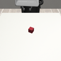
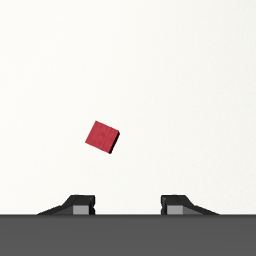
The task is marked as a success when the cube is lifted 5 centimetres above the table. Robosuite environments also support randomized initial states, which allows for diverse trajectories to be collected for training.

Data Collection

Training these JEPA world models requires a lot of data. In the original paper, for Push-T alone they used ~20,000 episodes with around 150 time-steps each. There was no existing dataset for the Robosuite Lift task and Robosuite had no scripted controllers built in, so I had to use teleoperation to collect data using a 3D SpaceMouse.

If you have ever used a SpaceMouse to control a robot, you know how terrible it is, and there was no way I was going to teleoperate 20,000 demos. Fortunately, Robosuite is compatible with MimicGen, which allowed me to expand a dataset of roughly 200 tele-operated episodes into 20,000 episodes with an average length of 72 time-steps.

The data collected for each episode consisted of RGB 84x84 frames recorded at 20Hz, along with proprioceptive state information consisting of the end-effector pose and the position of the gripper joints.

Evaluation

JEPA-based planning requires a goal state at inference time. In a full long-horizon system, a higher-level generative planner could theoretically sit above this low-level controller and generate intermediate goals from a desired task. Since this project focuses only on the low-level controller, I instead used demonstrations to provide the start and goal states for evaluation.

Rather than reusing training demonstrations, I tele-operated 50 fresh demonstrations that were never seen during training. For each evaluation rollout, I used the initial state from one of these demonstrations as the starting configuration and its final frame as the goal state.

World Model

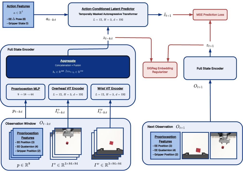
The “World Model” itself is split into an encoder and predictor, where the encoder condenses state observations into a latent representation. The predictor then learns how to estimate the next state within this latent space.

Encoder

The image encoder was a standard Vision Transformer with a patch size of 14, 12 layers, 3 heads, and an embedding dimension of 192. A small modification was made to the final output because generally the [CLS] token embedding outputted from the encoder is passed through a layer normalization. This interferes with the anti-collapse objective, which I explain more later. To prevent this, we add a projection layer with batch normalization after the layer normalization, which helps to “un-squish” the embedding.

Originally, I used shared weights between the agent-view and wrist-view encoders, but this led to really poor performance. Intuitively, this makes sense because the two views emphasize very different information. The agent-view camera provides features that describe object and robot positioning, whereas the wrist view provides finer-grained features that are useful for making small adjustments during grasping. That’s why I split the encoder into separate weights for each image.

Alongside these two image embeddings, I use a lightweight MLP to encode the proprioception state into a 64-dimensional embedding. This is then fused with the image embeddings to form the final state embedding, $z_t$:

$$h_t = [e_t^{agent}\; ;\; e_t^{wrist}\; ;\; e_t^{proprio}] \\[6pt] z_t = \operatorname{MLP}(h_t)$$

Predictor

This is a traditional causally masked autoregressive Transformer. It takes in a window of state embeddings, $z_{t-k:t}$, and predicts the next embedding, $\hat{z}_{t+1}$, similar to next-token prediction in LLMs. The predictor is also action-conditioned, so in addition to the window of state embeddings, it takes in a corresponding window of actions, $a_{t-k:t}$.

The action window is incorporated into the Transformer through Adaptive LayerNorm. These adaptive normalization layers replace the standard LayerNorms in the Transformer and allow the actions to modulate the latent prediction process. For a given embedding, $z$, Adaptive LayerNorm looks like this:

$$\operatorname{AdaLN}(z, a_{t-k:t})= \operatorname{LayerNorm}(z) \odot (1+\gamma) \ \ + \ \beta \\[6pt]\text{where } \gamma,\beta=\operatorname{MLP}_{\theta}(a_{t-k:t})$$

Training Objectives

In order to train accurate predictions, we use the MSE loss between the predicted next state, $\hat{z}_{t+1}$, and the true next state after being passed through the encoder, $z_{t+1}$:

$$\mathcal{L}_{\mathrm{pred}} = \left\| \hat{z}_{t+1} - z_{t+1} \right\|_2^2$$

Using this objective alone, however, would lead to representation collapse. This is when the encoder learns to minimize the loss by encoding every state into the same trivial embedding. To prevent this, we introduce an anti-collapse objective using Sketched Isotropic Gaussian Regularization (SIGReg).

This loss essentially measures how far a batch of embeddings outputted by the encoder diverges from an isotropic Gaussian distribution under random projections. Intuitively, this distribution forms a spherical cloud in the embedding space and encourages the representations to spread out instead of collapsing to a single trivial embedding.

SIGReg was introduced in LeJEPA, where the authors explore why this regularization is effective at preventing collapse while maintaining useful latent representations. In the final objective, this term is added to the prediction loss with a coefficient:

$$\mathcal{L}= \mathcal{L}_{pred} + \lambda \mathcal{L}_{SIGReg}$$

Frame Skips

In order to make the world model more effective over longer horizons, I use a frame skip (s). This means that successive observations used during training are actually (s) environment steps apart rather than coming from consecutive timesteps.

For example, with a frame skip of $s$ = 5 and a context window of $k$ = 3, the model would receive

$$z_t, z_{t-5}, z_{t-10}$$

and predict

$$z_{t+5}$$

This effectively lets each latent transition represent a longer period of motion. Since the robot action is 7-dimensional, each skipped transition also corresponds to an action chunk:

$$a \in \mathbb{R}^{s\times 7}$$

Planning in Latent Space

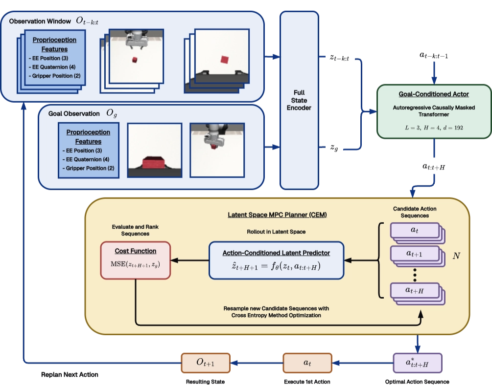
The original model predictive control method I used was Cross Entropy Method (CEM). I provide a more detailed algorithm below, but the gist of it is that the planner randomly samples a batch of action sequences over a horizon and then rolls them out using the world model. This results in an end state for each candidate sequence, which is scored using a cost function that measures how far it is from the goal state. The highest-ranking sequences are kept and used to fit a new distribution from which the next set of actions is sampled. This runs for a fixed number of iterations until the planner converges on a high-scoring action sequence, after which the first action from that sequence is executed and the planning phase restarts.

Temporal Straightening

In theory, CEM should work, but using MSE, which represents the Euclidean distance between the horizon state and the goal state, doesn’t always result in good trajectories. The reason is that, in latent space, the path from a starting state to a goal state isn’t always a straight-line interpolation between the two. More often than not, it is a curved path where the MSE does not consistently decrease throughout the trajectory. This can be seen in one of the successful demonstrations used during evaluation:

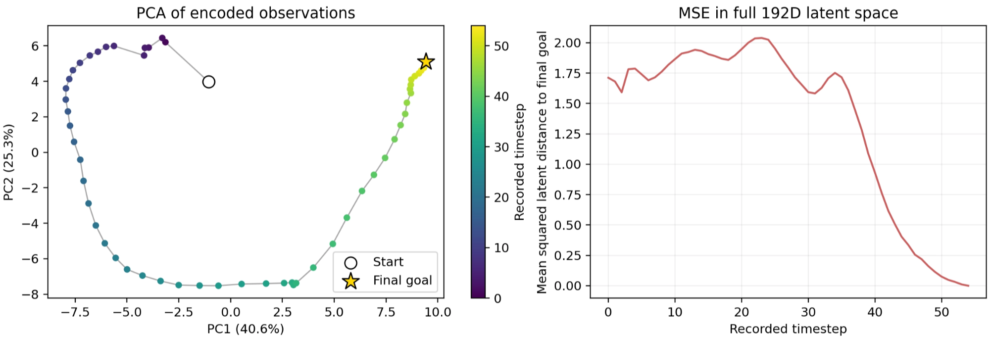
Wang et al. explored this in the paper Temporal Straightening for Latent Planning, where they introduced a training objective that maximized cosine similarity between subsequent embeddings. When I tried this, the prediction loss couldn’t converge to a nice value and the overall performance dropped drastically.

Goal-Conditioned Actor

To try and overcome this issue I trained a goal-conditioned actor policy concurrently with the world model, using the architecture from FlexiWorld. The actor is a small autoregressive Transformer conditioned on the current latent state, the goal state, and the previous action block.

More specifically, the actor uses the current state embedding, $z_t$, the difference to the goal, $z_g-z_t$, an elementwise interaction between the two, $z_t \odot (z_g - z_t)$, and the previous action block, $a_{t-1}$, as context. It then autoregressively predicts the next 5 actions, where each action is conditioned on the ones predicted before it. The actor is trained directly on demonstrated actions from the dataset using imitation learning.

To make the actor more robust at rollout, I also use Student Forcing for part of training. Instead of always conditioning on the ground-truth previous actions, the actor sometimes conditions on its own generated action prefix while still being supervised against the demonstrated actions.

At inference, the actor is combined with CEM using Actor-Residual CEM (ARCEM). Rather than searching directly over arbitrary action sequences, CEM searches over residual corrections to actions proposed by the actor. Importantly, these corrected actions are fed back into the actor as the imagined trajectory is rolled forward, so the actor continuously adapts its later proposals to the corrections made earlier in the sequence. The world model is then used to evaluate the resulting candidate trajectories and CEM iteratively refines the residual distribution.

Subgoal Scheduling

One limitation of latent world models is that prediction quality degrades as the rollout horizon gets longer. Because of this, I found it more effective to break the full Lift task into two shorter subgoals rather than always planning directly toward the final state. This better matches the world model’s strength at shorter-horizon prediction.

During training, each Robosuite demonstration contains metadata indicating the timestep at which the cube is successfully grasped. For samples before this grasp timestep, I use the grasp observation as the actor’s goal state. For samples at or after the grasp timestep, I instead use the final observation of the demonstration as the goal:

$$z_g = \begin{cases} z_{\text{grasp}}, & t < t_{\text{grasp}} \\ z_{\text{final}}, & t \ge t_{\text{grasp}} \end{cases}$$

At inference, I follow the same two-stage structure. The rollout begins with the grasp frame as the active goal and the controller is given a fixed budget of 50 environment timesteps to reach it. Since each planner output executes a 5-action chunk, this corresponds to 10 replanning cycles. Once this budget is exhausted, the active goal switches to the final demonstration frame and the controller is given another fixed budget before the rollout terminates.

Experiments

In order to evaluate the model and different aspects of the system, I ran all 50 evaluation demonstrations across several configurations that varied the control algorithm, actor usage, and encoder setup. I also measured the planning time per action chunk to estimate the maximum effective control frequency.

Ablations

All of these configurations were trained with a frame skip of 5, resulting in action chunks of 5 steps, and with a planning horizon of 5.

Configuration	Planner	Encoder	Samples (N)	Elites (K)	Iterations (I)	Temperature (tau)
Shared-Encoder CEM	CEM	Shared	600	30	10	—
Normal CEM	CEM	Split	600	30	10	—
Direct	Actor only	Split	—	—	—	—
Small ARCEM	ARCEM	Split	128	16	3	0.5
Medium ARCEM	ARCEM	Split	200	20	5	0.5
Normal ARCEM	ARCEM	Split	600	30	10	0.75

Results

Configuration	Success Rate	Planning Time / Chunk	Max. Effective Control Frequency
Shared-Encoder CEM	28%	0.352 s	14.2 Hz
Normal CEM	40%	0.352 s	14.2 Hz
Direct	38%	0.091 s	54.9 Hz
Small ARCEM	88%	0.389 s	12.9 Hz
Medium ARCEM	80%	0.606 s	8.3 Hz
Normal ARCEM	78%	1.47 s	3.4 Hz

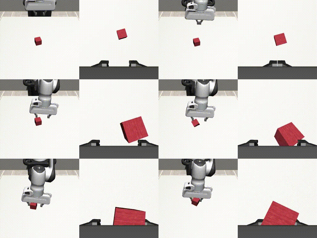
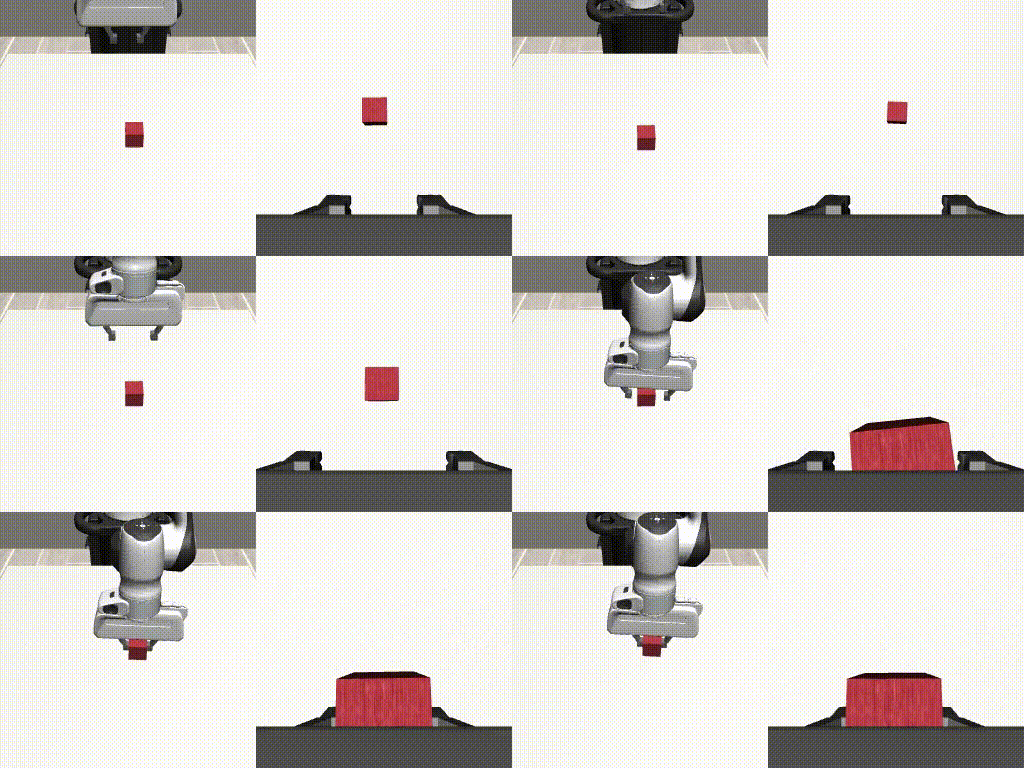
Failures and Limitations

Although I was able to train a successful policy with this approach, there are still several major drawbacks:

• Very data hungry: Roughly 20,000 demonstrations is a lot of data for a relatively simple task like Lift. A behavioural cloning policy could likely learn the same task with far less data.
• Explicit goals and subgoals: I manually split the task into grasping and lifting and used demonstration frames as the goals. This works here, but a more general system would need to generate or discover these intermediate goals automatically.
• Privileged goal information: The grasp and final goal observations come directly from successful demonstrations, which obviously would not be available during a real deployment.
• High planning latency: MPC requires repeatedly evaluating many imagined trajectories, and combining this with autoregressive neural networks makes planning relatively slow.

Takeaways and Next Steps

The biggest thing I took away from this project is that world models can definitely be useful for robot control, but there is still a lot left to figure out before they become practical for general manipulation.

One obvious next step is replacing the manually defined subgoals with a higher-level planner that generates intermediate goals for the low-level controller. The actor would also need to become more robust to a wider variety of goals, potentially by randomizing the future goal state used during training. A recently released paper, H-JEPA, looks especially relevant to this direction.

I also think world models may end up being more useful beyond directly planning with MPC. I was talking with someone working in the field about this, and they made an interesting point: when you optimize actions directly through a learned world model, the planner may find trajectories that exploit inaccuracies in what the model predicts will work. If the model has weaknesses, MPC can end up taking advantage of them rather than producing genuinely good behaviour.

An alternative is to let a policy generate the actions and use the world model mainly to simulate and evaluate the resulting rollouts. In that setup, the model is being used more as a learned simulator than as something the controller directly optimizes against. That could be really useful for accelerating reinforcement learning, testing policies cheaply, or reducing the amount of real-world evaluation needed before deployment.

I still want to keep exploring this space, especially with larger architectures, generative dynamics models such as flow matching, and harder manipulation tasks like pick-and-place or eventually dexterous assembly.